EM Algorithm on linear model clusters in R
Let’s together explore another technique that it has several application which includes parameter estimation on mixtures models or hidden markov models, data clustering, and discovering hidden variables - EM Algorithm applications. To grasp the power of EM-Algorithm let’s considered an always familiar and simple linear models, and try to discover from which model was the points originated (clustering) with an iterative approach.
This is a crosspost from EM with mix of two linear models, with some personal changes to the original code.
The algorithm basically solve the following problem: given a set of observations and prior knowledge of how many distributions generated the observations, is it possible to estimate from which observation belongs to which distribution?.
Generate random data
Create a function that generates observation based on a linear model with some gaussian noise:
# The noise, number of observation and even the spread of these observation can all be customize
  observation.random_lm <- function(slope,intercept, noise=0.35, N=40, upper_x=501) {
    xs <- sample(seq(-5,10,len=upper_x), N)
    ys <- intercept + slope*xs + rnorm(length(xs),0,noise)
    cbind(xs,ys)
  }
To use and plot:
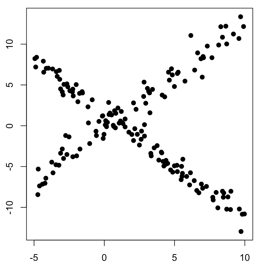
mydata <- rbind( random_lm(-1.3,1.5,noise=0.85,N=100, ), random_lm(1.3,-0.5, N=75, noise=1.2) )
png("em-0.png", width=900, height=570, units="px", pointsize=18)
plot(mydata, pch=19, xlab="X", ylab="Y")
title("EM Maximization for Linear models initial")
Now the image bellow just by simple sight two different linear pattern emerge, so the EM algorithm is used to find the hyperparameters that generated these distribution automatically.
Pseudo code of the EM-Algorithm
Step 1: Initialize random parameters
Since here, there is prior knowledge of 2 distributions the parameters that need to be generated are:
\[f_1(x) = \beta_0 + \beta_1X\] \[f_2(x) = \beta_1 + \beta_2X\]Assuming some uniform distribution to randomly initialize these \(\beta_n\) we have:
init_params <- function() {
  i1 <<- 2*runif(1)
  s1 <<- 2*runif(1)
  i2 <<- 2*runif(1)
  s2 <<- 2*runif(1)
  c(i1,s1,i2,s2)
}
Step 2: Calculate each observation probabilities
With the initialization parameters, let’s proceed to calculate the weights of each observation assuming a gaussian noise is present:
e.step <- function(mydata, params, sigma=0.75) {
  e1 <- exp( (-abs(params[1] + params[2]*mydata[,1] - mydata[,2])^2)/(sigma^2) )
  e2 <- exp( (-abs(params[3] + params[4]*mydata[,1] - mydata[,2])^2)/(sigma^2) )
  cbind(e1/(e1+e2), e2/(e1+e2))
}
Now is a matter to use these calculated weight to solve using Weighted Least Square
wls <- function(X,Y,W) {
  solve(t(X) %*% W %*% X) %*% t(X) %*% W %*% Y
}

### Step 3: Use the weighted parameters and recalculate the parameters

m.step <- function(mydata, ws) {
  X <- cbind(rep(1, nrow(mydata)), mydata[,1])
  Y <- as.matrix(mydata[,2], ncol=1)
  p_1 <- wls(X,Y,diag(ws[,1]))
  p_2 <- wls(X,Y,diag(ws[,2]))

  c(p_1, p_2)
}
As a side note is important to now that the solve function will calculate the inverse of the formula inside it..
We can use both the e.step and m.step functions iteratively to calculate the parameters continuously until it converged, or it reached a max of iterations.
EM Algorithm for linear model steps by step: