
Text classification modelling with tidyverse, SVM vs Naivebayes
It’s been a while since I wrote something, years actually, but here we go. Modelling is at the core of statistical learning, it allows us to make use of different techniques usually to predict, classify or find pattern within a particular dataset. USually the workflow involves a preprocessing with several tecniques and decision, such as imputation, omitting na, normalization, centering, and so on. Here I want to explore how the tidyverse has created an ecosystem that allows for fast and simple use of different modelling for comparison.
This post is inspired on: A guide to Text Classification(NLP) using SVM and Naive Bayes with Python but with R and tidyverse feeling!
Dataset
The dataset is Amazon review dataset with 10K rows, which contains two label per review __label1 and __labe2 which we will use to compare two different models for binary classification.
Text classification
Text classification is one of the most common application of machine learning. It allows to categorize unstructure text into groups by looking language features (using Natural Language Processing) and apply classical statistical learning techniques such as naive bayes and support vector machine, it is widely use for:
-
Sentiment Analysis: Give a text which could be a comment, review, a tweet, or a post inferred what feeling it’s expressing at the moment, it can provide a lot of insight into how a customer based is perceiving your brand at the moment.
-
Language detection Give a text to be able to detect the language can be a useful tool on the first stages of a multi-language translation tool like google translate.
Hands on example
Overall machine learning looks very similar to the figure bellow, there are severa process before trying out different models, and usually involve a number of nuances and tecnique in order to set the data in a state that is friendly towards a particular model. Here the focus is on working with unstructure text and extracting features out of it.
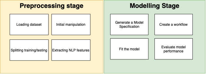
Preprocessing stage
1.1 Loading dataset
This is rather obvious but in order to work on the dataset there need to be a source to which it can be fetch. In this case the dataset is sufficiently small to be able to work on memory but other type of data may require more sophisticated approaches.
loading_data <- function(path) {
  readr::read_csv(path, locale = locale(encoding = "latin1"))
}
The parameter for locale is important because the corpus.csv has been encoding with latin character into it.
1.2 Initial manipulation of data
Usually when working with classification one needs to identify those records that are not beeing classify correctly and explore what is the underlying reason behind it, as a good practice one can use the initial row number as a surrogate Id when one does not explicitly exist, so the initial manipulation of data follows two steps, identify the records by adding an Id column and omit the empty or NA records.
corpus <- loading_data("svm_textclassification/corpus.csv") %>%
          mutate(Id = row_number(), label = factor(label)) %>%
          na.omit()
1.3 Splitting training and testing subset
This is very easy to achieve in R thanks to rsample package it’s basically a matter to create an initial split and reuse it in order to create two different subset randomly selected.
text_split <- initial_split(corpus)
training_set <- training(text_split)
test_set <- testing(text_split)
1.4 Extracting NLP features
Now let’s talk about some features that we intent to use in order to create a design matrix later on.
- Tokenize the text: Since the classification will depend on a sequence of words, tokenization refers to a mechanism to split this words as individual and atomic unit call tokens. The standards way to split this in indo-european language is through spaces although this can result to some strange token that may not be necesarilly useful.
- Remove stopwords: this refers to words that have a high frequency within a corpus usually articles, pronouns, common verbs, adjective. Commonaly when working with statistical model this words do not provide additional information, therefore get remove from before providing to the model. Of course each language has different stopwords and they also can get customize depending on the nature of the corpus to be work on. Read further about this on Stop words wikipedia
- Lemmatization: A lemma in NLP it’s a root of a words, considering that in languages one word have multiple ways to be written, for instance: study, studying, studied may benefit the model to work on a single unit rather than use then as three independent words. Standford stemming and lemmatization
- Term Frequency, Inverse Document Frequency (TF-IDF) : is a statistical method in order to score the importance of a words based on the its frequency within a specific document and the overall corpus to be analyze. It is a very commmon technique on information retrieval and text mining, for its simplicity on providing a relatively solid base for ranking search terms. The math behind it is very simple but it’s outside the scope of this guide, if you are interested in reading further: TF-IDF on wikipedia
It seems like a lot but tidyverse has a nice package recipes that helps in create a series of steps for all the above preprocessing of the text. This is a snippted on how can this be achieve:
text_recipe <- recipe(label ~ ., data = training_set) %>%
  update_role(Id, new_role = "ID") %>%
  step_tokenize(text, engine = "spacyr") %>%
  step_stopwords(text) %>%
  step_lemma(text) %>%
  step_tokenfilter(text, max_tokens = 100) %>%
  step_tfidf(text)
Modelling stage
Once the preprocessing has been apply to our dataset it’s time to move to the modelling phase, given that this is just an example we’re going to compare two different statistical models Naive Bayes and Support Vector Machine without any hyperparameter tunning or cross validation tecniques. The main purpose is how to specify this models in a plug and play way using parnsnip + workflow and evaluate their performance using yardstick.
2.1 Create model specificatoin
A very straight forward step thanks to parnsnip if you are familiar with caret it serves a similar purpose although with a tidy feeling into it. parsnip A tidy model interface - Max Kuhn explained in greater detail the idea behind it.
text_model_NB_spec <- naive_Bayes() %>% set_engine("naivebayes") %>% set_mode("classification")
text_model_svm_spec <- svm_poly("classification") %>% set_engine("kernlab")
2.2 Create workflow
Workflow is a very interesting package I recently stumble upon from tidymodels, basically serve as a bridge between the recipe instruction for preprocessing and the model specification, it can be use a sort of plug and play kind of technique where the model can be replace easily by providing a different specification. Hopefully I’ll soon write a way to exploit this to run hyperparameters tunning. In the meantime this is the tecnique use for this example:
text_model_NB_wf <- workflows::workflow() %>% add_recipe(text_recipe) %>% add_model(text_model_NB_spec)
text_model_svm_wf <- workflows::workflow() %>% add_recipe(text_recipe) %>% add_model(text_model_svm_spec)
As you can see the recipe object remains the same accross both workflow and the model specification differs from Naive bayes to support vector machine.
2.3 Fit the model
Finally the fittin of the model starts, here there won’t be any cross validation or resampling tecnique in use, instead we can basically start fitting the model right on.
fit_NB_model <- fit(text_model_NB_wf, training_set)
fit_svm_model <- fit(text_model_svm_wf, training_set)
2.4 Evaluate model performance
Be able to measure the performance of any type of machine learning is crucial in order to select the right model for the job. Sometime selecting which measures to use can be tricky but here is very straighforward we’ll look on how to built a confusion matrix and measure accuracy, aswell as ROC curve and ROC AUC for a better view.
Confusion matrix and accuracy
Confusion matrix organize the results depending on the prediction and the truth value of the observation, this allows to view wether the model is classifying correctly the testing set, confusion matrices also allow to calculate other measurement for the classification like accuracy, sensitivity and recall.
predictions_NB <- predict(fit_NB_model, test_set)
predictions_SVM <- predict(fit_svm_model, test_set)

bind_cols(test_set,predictions_NB) %>% conf_mat(label, .pred_class)
bind_cols(test_set,predictions_NB) %>% accuracy(truth = label, estimate = .pred_class)
ROC Curve and ROC AUC
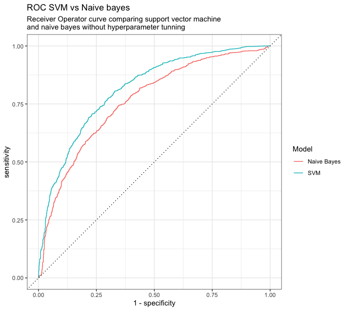
Another more proper way to analyze the performance of binary classification models is the use of ROC AUC and ROC Curve, the former provides a number of how much area under the curve is explained by the model and the latter a visual representation of how well the models works in different threshold of classification.
roc_NB <- bind_cols(test_set,prediction_NB_prob) %>% roc_curve(label, .pred___label__1) %>% mutate(Model="Naive Bates")
roc_SVM <-  bind_cols(test_set,prediction_SVM_prob) %>% roc_curve(label, .pred___label__1) %>% mutate(Model="SVM")

bind_rows(roc_NB,roc_SVM) %>%
  ggplot(aes(x = 1 - specificity, y = sensitivity, color=Model)) +
  geom_path() + geom_abline(lty = 3) +
  coord_equal() + theme_bw() +
  ggtitle("ROC SVM vs Naive bayes","Receiver Operator curve comparing support vector machine \nand naive bayes without hyperparameter tunning")
Conclusion
Machine learning can be an overwhelming task, it require several steps in order to start modelling and testing. Tidy models and tyidtverse are a great way to accomplish statistical analysis and modelling without too much hassle, of course one still needs to understand both which tecnique to use and understand tidy principles in order to make the best use of it. But for this particular scenario the use of SVM is providing a better explanation for the dataset, there’s still a lot of more tuning that can be done in order to improve upon this tecnique. The overall purpose was to provide a way to show how all of these packages work together to help out in the process of modelling our data.
Packages and their purpose
Most of the packages are part of the tidyverse umbrella, all of them play very nice with each, and serving a particular purpose rather well.
- readr Provides an easy interface to read csv files.
- dplyr It aid to manipulate data easily with function like
filter(),summarise(),arrange()and with its pipe like flow that improves readibily of code. - recipes Use to create design matrices for modelling and some data preprocessing through a step base functions.
- yardstick Contains several functions to measure how well a model performs.
- parsnip It’s a middle layer to easily plug-and-play different modelling packages within a single programming interface.
- textrecipes Expand the recipe package for some basic NLP features and preprocessing.
- workflows Help to bundle together recipes and modelling in order to plug them by demand.
- rsample Useful for sampling and resampling technique as well as splitting dataset among training/testing
- ggplot2 To create graphics declarative base on Grammar of Graphics.
- discrim Model Wrappers for Discriminant Analysis.
- kernlab Kernel Based Machine learning lab
Code
All the code describe here can be found on text_classification.R
Sessioninfo
R version 3.6.2 (2019-12-12)
Platform: x86_64-apple-darwin15.6.0 (64-bit)
Running under: macOS Catalina 10.15.4

Matrix products: default
BLAS:   /System/Library/Frameworks/Accelerate.framework/Versions/A/Frameworks/vecLib.framework/Versions/A/libBLAS.dylib
LAPACK: /Library/Frameworks/R.framework/Versions/3.6/Resources/lib/libRlapack.dylib

locale:
[1] en_US.UTF-8/en_US.UTF-8/en_US.UTF-8/C/en_US.UTF-8/en_US.UTF-8

attached base packages:
[1] stats     graphics  grDevices datasets  utils     methods   base

other attached packages:
[1] dplyr_1.0.0

loaded via a namespace (and not attached):
[1] Rcpp_1.0.4.6      rstudioapi_0.11   magrittr_1.5      hms_0.5.3         tidyselect_1.1.0  doParallel_1.0.15
[7] R6_2.4.1          rlang_0.4.6.9000  foreach_1.5.0     fansi_0.4.1       tools_3.6.2       parallel_3.6.2
[13] packrat_0.5.0     utf8_1.1.4        cli_2.0.2         iterators_1.0.12  ellipsis_0.3.0    assertthat_0.2.1
[19] tibble_3.0.1      lifecycle_0.2.0   crayon_1.3.4      purrr_0.3.4       readr_1.3.1       vctrs_0.3.1
[25] codetools_0.2-16  glue_1.4.0        compiler_3.6.2    pillar_1.4.3      generics_0.0.2    renv_0.9.3
[31] pkgconfig_2.0.3