Behind the curtains on montecarlo sampling methods
Recently I’ve been going through the incredible book by Prof Elreath on statistical rethinking; it’s quite a good book to wrap your head around bayesian approach on causual analysis, as the book progress and starts to stack more and more concept together it reaches a point where a more sophisicated approach to sample the posterior probability will be required. Hence by the
I have been particularly fond of the explanation on Markov Chain montecarlo and its application, it is without a doubt one of the most comprehensive introduction to such methods, the king analogy for Metropolis (refered as Rosenbluth), all the way through hamiltonian approach on sampling posterior distributions and the use of a physics simulation (the gradient calculation).
Here is a quick recap of what I consider the most substantial explanation of this chapter, along with some additional links to further learn about the subject.
The benevolant Markov King

As explained the algorithm is very straight forward, the goal of Markov king is to visit each island to which he ruled proportional to the population size of each island the bigger the population the more the king will stay or visit it. So metropolis algorithm recipes goes like this:
- Randomly pick an island as the inital point, for the purposes of this example this could be deterministic (i.e population size).
- Flip a coin (bernoulli event) 50/50 what’s the next island to consider left or right.
- Now (an this is the crucial part) in order to move the king to the proposal island, here we basically run a uniform distribution with probability p, which is a ratio of the proposal island population over the current island population.
- Repeat
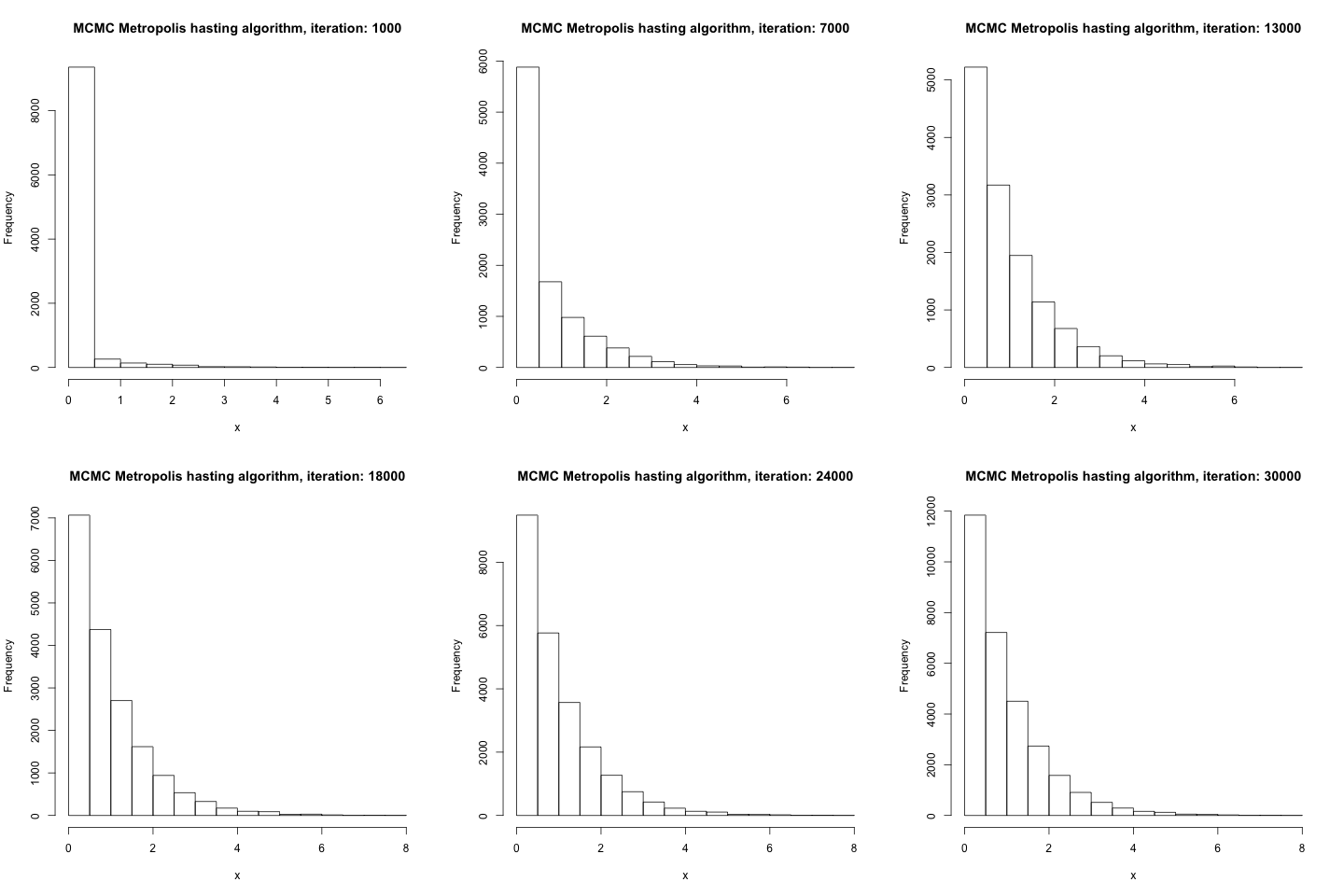
Now this might not sounds like anything but after running graphically what’s going, you can convinced yourself that this approach actually converge to the initial goal of “visiting an island depending on the population size”
Graphical simulation of Metropolis Algorithm

Let’s code this up!
On R code the algorithm would look something like this.
num_weeks <-  1e6
position <- rep(0, num_weeks)
current <- 10
for (i in 1:num_weeks) {

  position[i] <- current
  proposal <- current + sample( c(-1, 1), size = 1)
  if (proposal < 1) proposal <- 10
  if (proposal > 10) proposal <- 1

  prob_move <- proposal/current
  current <- ifelse(runif(1) < prob_move, proposal, current)
}

plot(table(position))
- First we are setting everything up, simulation a million weeks (
num_weeks <- 1e6), creating an array fill with zeros of length 1e6 (position <- rep(0, num_weeks), and setting an arbitrary island to startcurrent <- 10 - Now iterate and the most important part here is the proposal, after we sample
sample( c(-1, 1), size = 1)basically flipping a coin to go left or right. - The
if (proposal < 1)and ` if (proposal > 10)` are there only to ensure we’ll circle the island on the edges so when we reached an island bigger than 10 (i.e ) index we’ll treat it as 1 and if we get an island index smaller than 1, we’ll go to 10. - Now we use the proposal and the current to have a probability to move or stay ` prob_move <- proposal/current`
- Then based on the proportion of the probability we decide to move
current <- ifelse(runif(1) < prob_move, proposal, current)
At some point this will converge to the right distribution, so island that are big will be visited more and appear more frequen in the position array than island with smaller population.
About gibbs sampling and asymetric proposals
Metropolis is a rather easy algorithm to explained but it is not without its limitation, so it would work to jump from one island to the other when this distribution is symetric, but this is not always the case. Metropolis-Hasting do allow for asymetric probabilities which following the king markov analogy we would have a biased coin based on which island is visited; a special case for metropolis-hasting is known as GIBBS sampling that allow us to sample proposal more efficiently, leveraging what it called adaptive proposal where the distribution proposed parameter adjust itself depending on the parameters at the moment.
If the statement above confused you., you’re not alone it confused me too, let’s see how gibbs handling these adaptive parameters with a graphical example:

Graphical tool for different Monte carlo methods https://chi-feng.github.io/mcmc-demo/app.html
That’s it for now
We’ll leave it here as this post had become a bit too long for my taste, I’ll comeback with an explanation on HMCM, and some real world applications.