
Predicting a legendary pokemon through Logistic regression in R
Recently I stumble with a pokemon dataset, and for anyone growing up in the 2000’s this brough up good memories, so of course I decided to take a peek into it. Let’s try to use logistic regression for predicting wether a pokemon would be a legendary based on features available, in the process we can look at how quickly explore the dataset with ggplot, splitting on training/testing, work with imbalance classes and looking at the result.
Exploratory data analysis
As usual, the starting point is to understand the dataset, this can be achieve visually through different type of plots, or calculating numeric values of interest such as frequencies or correlation values. In general though there is some sort of documentation or previous knowledge of what we’re dealing with, in this case as it is a kaggle dataset there is plenty information about the information each columns provide. For example:
name: The English name of the Pokemon
japanese_name: The Original Japanese name of the Pokemon
pokedex_number: The entry number of the Pokemon in the National Pokedex
percentage_male: The percentage of the species that are male. Blank if the Pokemon is genderless.
type1: The Primary Type of the Pokemon
type2: The Secondary Type of the Pokemon
classification: The Classification of the Pokemon as described by the Sun and Moon Pokedex
.....
This give us an idea into how to treat some of our columns, by default unlike data.frame (although recently changed) readr, will NOT automatically transform character columns into factors, therefore some aditional treatment need to be made in order to accomodate some columns before examining. In this stage of preprocessing it is require to go through each column (or at least those that are of interest for the modelling and analysis), althought this is unfeasable when dealing with dataset with large amount of features. Again the code to initially mutate the dataset to our will looks like this:
map_fn <- function(x) {
  length(str_split(x, ",", simplify = TRUE))
}

get_maximum_abilities <- function(pokemon_df) {
  pokemon_df %>% pull(abilities) %>% map_int(map_fn) %>% max()
}

clean_ability <- function(ability) {
  gsub("\\[|\\]|\\'","", ability)
}

pokemon_df <- pokemon_data %>% na.omit() %>%
    mutate(abilities = clean_ability(abilities)) %>%
    separate('abilities', paste0("ability",1:max_abilities), sep=',') %>%
    mutate(is_legendary = factor(is_legendary),
           type1 = factor(type1), generation = factor(generation)) %>%
    mutate_at(vars(starts_with("ability")), factor) %>%
             select(-starts_with("against"))
Very straightforward the first lines are splitting the abilities column into several other columns using the separate function, next transform both the is_legendary and type1 to factors, and finally dropping columns that are not likely of interest or to cumbersome to deal with. Great now there are several ways to move forward, one of my favorite is leveraging the usage of a package in R called skimr that basically provide several values of interest per column.
skimr::skim(pokemon_df)
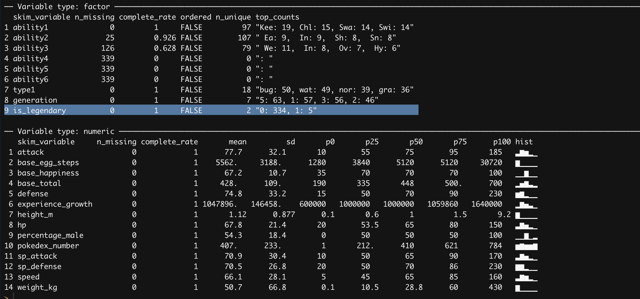
Looking at the summary statistic skimr provides there is a major problem of class imbalance with our target variable. Even though we are going to use logistic regression which is shield it from class imbalance there are so few datapoints of legendary pokemon to work with. Before addressing this issue, let’s look visually how do our numeric features correlate with each other
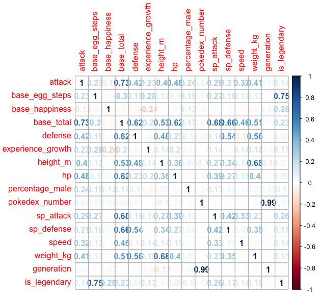
Here we can see some correlation through between the features, for instance: attack, defense and speed are correlated with based total, there is of course generation and pokedex number are highly positive correlated but it’s unlikely to yield any information regarding the legendary nature of a pokemon, for obvious reason.
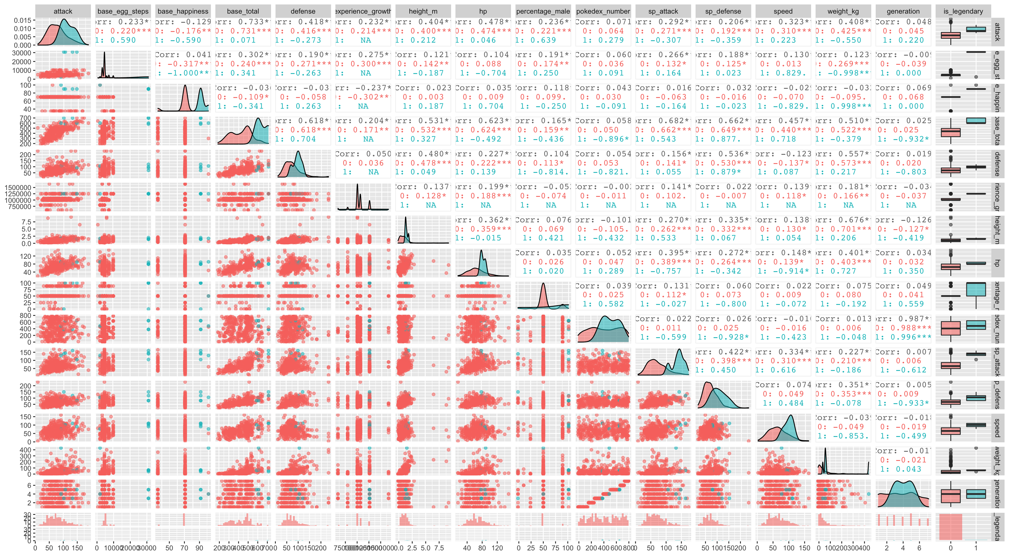
Another interesting way to look at several columns relation at a time is to use ggplot extension package called GGally similarly to skimr aggregate and combine several statistic into interest plots, such as distribution plots, correlation matrices, pairwise plot matrices, box plot and so on.
pokemon_data %>% na.omit() %>%
  select_if(~ is_double(.x) | is_integer(.x)) %>%
  select(-starts_with("against")) %>%
  mutate(is_legendary = factor(is_legendary)) %>%
  ggpairs(aes(color = is_legendary, alpha = 0.8))
Similar to corrplot function ggAlly spits out correlation plot in the upper triangular and the scatter plot in the lower triangular, again the challenge here is the lack of sample of legendary pokemons, so its’ now time to address this in the modelling phase.
Applying logistic regression
First thing first! split the data is crucial, unfortunately the data imbalance it’s a challenge as we won’t be able to built a proper model, so in order to address this issue we’ll be looking to use an algorithm to perform over sampling called SMOTE (synthetic minority over-sampling technique). Now it’s true that regression models for classification do not exhibit issues when it comes to class imbalance it’s also true that so few datapoints will pose a challenge for a classification perspective. The package DMwR has a nice implementation of SMOTE algorithm in R and very straighforward once we split training and testing, we’ll use training for generating synthetic data.
pokemon_split <- initial_split(pokemon_design, strata = is_legendary)
training_pokemon <- training(pokemon_split)
testing_pokemon <- testing(pokemon_split)
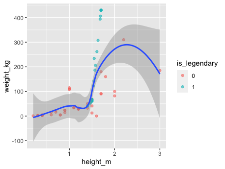
smoted_training_pokemon <- SMOTE(is_legendary ~ ., as.data.frame(
select_if(training_pokemon, ~is_numeric(.x))),
perc.over = 500, k = 2) %>% na.omit() SMOTE basically work with a nearest neighbors in order to generate data that look as much as possible to the original dataset, one need to be careful with the selection of k usually it is a higher number, but given that the dataset contains so few points it’s therefore necesary to have a lower number. Here is a result ilustrated the synthetic data generated:
In order to run logistic regression glmnet it’s the go to package, as usual it provides as many other model algorithm in R an implementation of the fit method, once X design matrix and y target values is provided it will do the rest. As shown bellow:
x <- data.matrix(smoted_training_pokemon %>% select(-is_legendary))
y <- smoted_training_pokemon$is_legendary
# Simply using glmp for classification no recipe or no workflow or tunnning just yet
fit = cv.glmnet(x, y, family = "binomial")

pred = predict(fit, data.matrix(testing_pokemon %>%  select_if(is_numeric) %>% select(-is_legendary)),
        type = "class", s = 'lambda.min' )

bind_cols(.pred = pred, testing_pokemon) %>%
  mutate(correct = .pred == is_legendary) %>%
  ggplot(aes(x = height_m, y = weight_kg, color = .pred, shape = correct)) +
  scale_shape_manual(values=c(4, 19)) +
  geom_point(alpha = 0.8, size = 3)

# Confusion matrix
bind_cols(.pred = pred, testing_pokemon) %>%
  mutate(correct = case_when(.pred == is_legendary ~ 1, T ~ 0)) %>%
  select(is_legendary, .pred) %>% table()